Sequential Monte Carlo
Introduction
Arguably the core of QInfer, the qinfer.smc module implements the
sequential Monte Carlo algorithm in a flexible and robust manner. At its most
basic, using QInfer’s SMC implementation consists of specifying a model, a
prior, and a number of SMC particles to use.
The main component of QInfer’s SMC support is the SMCUpdater class,
which performs Bayesian updates on a given prior in response to new data.
In doing so, SMCUpdater will also ensure that the posterior particles
are properly resampled. For more details on the SMC algorithm as implemented
by QInfer, please see [GFWC12].
Using SMCUpdater
Creating and Configuring Updaters
The most straightfoward way of creating an SMCUpdater instance is to
provide a model, a number of SMC particles and a prior distribution to choose
those particles from. Using the example of a SimplePrecessionModel,
and a uniform prior \(\omega \sim \text{Uni}(0, 1)\):
>>> from qinfer import SMCUpdater, UniformDistribution, SimplePrecessionModel
>>> model = SimplePrecessionModel()
>>> prior = UniformDistribution([0, 1])
>>> updater = SMCUpdater(model, 1000, prior)
Updating from Data
Once an updater has been created, one can then use it to update the prior distribution to a posterior conditioned on experimental data. For example,
>>> true_model = prior.sample()
>>> experiment = np.array([12.1], dtype=model.expparams_dtype)
>>> outcome = model.simulate_experiment(true_model, experiment)
>>> updater.update(outcome, experiment)
Drawing Posterior Samples and Estimates
Since SMCUpdater inherits from Distribution,
it can be sampled in the same way described in Representing Probability Distributions.
>>> posterior_samples = updater.sample(n=100)
>>> posterior_samples.shape == (100, 1)
True
More commonly, however, one will want to calculate estimates such as
\(\hat{\vec{x}} = \mathbb{E}_{\vec{x}|\text{data}}[\vec{x}]\). These
estimates are given methods such as est_mean() and
est_covariance_mtx().
>>> est = updater.est_mean()
>>> print(est)
[ 0.53147953]
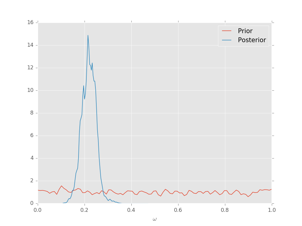
Plotting Posterior Distributions
The SMCUpdater also provides tools for producing plots to
describe the updated posterior. For instance, the
plot_posterior_marginal() method uses kernel
density estimation
to plot the marginal over all but a single parameter over the posterior.
prior = UniformDistribution([0, 1])
model = SimplePrecessionModel()
updater = SMCUpdater(model, 2000, prior)

# Plot according to the initial prior.
updater.plot_posterior_marginal()

# Simulate 50 different measurements and use
# them to update.
true = prior.sample()
heuristic = ExpSparseHeuristic(updater)

for idx_exp in range(25):
    expparams = heuristic()
    datum = model.simulate_experiment(true, expparams)
    updater.update(datum, expparams)

# Plot the posterior.
updater.plot_posterior_marginal()

# Add a legend and show the final plot.
plt.legend(['Prior', 'Posterior'])
plt.show()
(Source code, svg, pdf, hires.png, png)

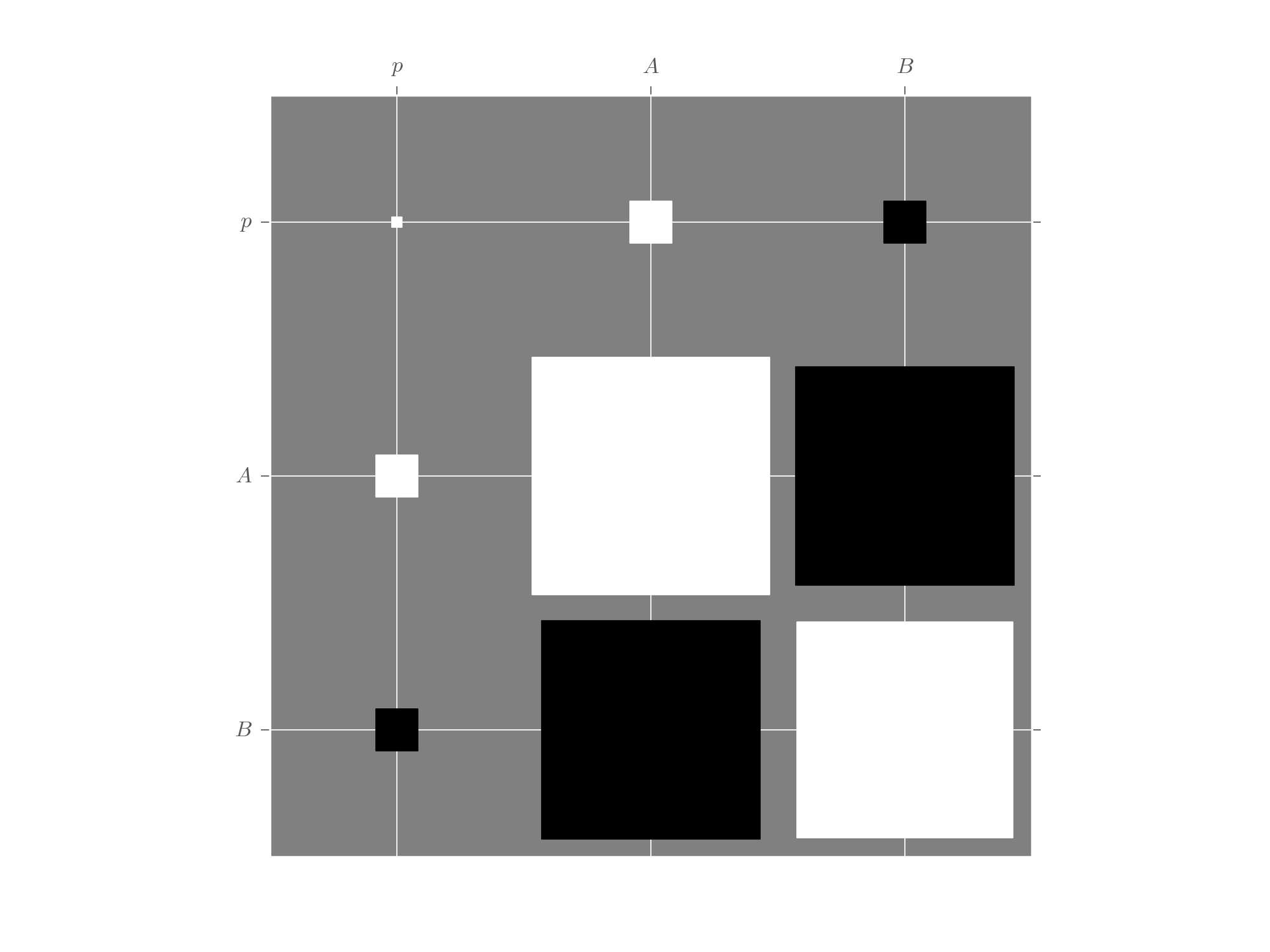
For multi-parameter models, the plot_covariance()
method plots the covariance matrix for the current posterior
as a Hinton diagram.
That is, positive elements are shown as white squares, while negative elements
are shown as black squares. The relative sizes of each square indicate the
magnitude, making it easy to quickly identify correlations that impact estimator
performance. In the example below, we use the Simple Estimation Functions to
quickly analyze Randomized Benchmarking data and show the resulting correlation
between the \(p\), \(A\) and \(B\) parameters. For more detail,
please see the randomized benchmarking example.
p = 0.995
A = 0.5
B = 0.5

ms = np.linspace(1, 800, 201).astype(int)
signal = A * p ** ms + B

n_shots = 25
counts = np.random.binomial(p=signal, n=n_shots)

data = np.column_stack([counts, ms, n_shots * np.ones_like(counts)])
mean, cov, extra = simple_est_rb(data, return_all=True, n_particles=12000, p_min=0.8)
extra['updater'].plot_covariance()

plt.show()
(Source code, svg, pdf, hires.png, png)

Advanced Usage
Custom Resamplers
By default, SMCUpdater uses the Liu and West resampling algorithm [LW01]
with \(a = 0.98\). The resampling behavior can be controlled, however, by
passing resampler objects to SMCUpdater. For instance, if one wants to
create an updater with \(a = 0.9\) as was suggested by [WGFC13a]:
>>> from qinfer import LiuWestResampler
>>> updater = SMCUpdater(model, 1000, prior, resampler=LiuWestResampler(0.9))
This causes the resampling procedure to more aggressively approximate the posterior as a Gaussian distribution, and can allow for a much smaller number of particles to be used when the Gaussian approximation is accurate. For multimodal problems, it can make sense to relax the requirement that the resampler preserve the mean and covariance, and to instead allow the resampler to increase the uncertianty. For instance, the modified Liu-West resampler \(a = 1\) and \(h = 0.005\) can accurately find exactly degenrate peaks in precession models [Gra15].
Posterior Credible Regions
Posterior credible regions can be found by using the
est_credible_region() method. This method returns a set of
points \(\{\vec{x}_i'\}\) such that the sum \(\sum_i w_i'\) of the
corresponding weights \(\{w_i'\}\) is at least a specified ratio of the
total weight.
This does not admit a very compact description, however, such that it is useful to find region estimators \(\hat{X}\) containing all of the particles describing a credible region, as above.
The region_est_hull() method does this by finding a convex
hull of the credible particles, while region_est_ellipsoid()
finds the minimum-volume enclosing ellipse (MVEE) of the convex hull region
estimator.
The derivation of these estimators, as well as a detailed discussion of their performances, can be found in [GFWC12] and [Fer14].
Online Bayesian Cramer-Rao Bound Estimation
TODO
Model Selection with Bayes Factors
When considering which of two models \(A\) or \(B\) best explains a
data record \(D\), the normalizations of SMC updates of the posterior
conditoned on each provide the probabilities \(\Pr(D | A)\) and
\(\Pr(D | B)\). The normalization records can be obtained from the
normalization_record properties of each. As the
probabilities of any individual data record quickly reach zero, however, it
becomes numerically unstable to consider these probabilities directly. Instead,
the property log_total_likelihood records the quantity
for \(M \in \{A, B\}\). This is related to the Bayes factor \(f\) by
As discussed in [WGFC13b], the Bayes factor tells which of the two models under consideration is to be preferred as an explanation for the observed data.