Quantum Tomography
Introduction
Tomography is the most common quantum statistical problem being the subject
of both theoretical and practical studies. The qinfer.tomography module
has rich support for many of the common models of tomography including
standard distributions and heuristics, and also provides convenient plotting
tools.
If the quantum state of a system is \(\rho\) and a measurement is obtained, then the probability of obtaining the outcome associated with effect \(E\) is \(\operatorname{Pr}(E|\rho) = \operatorname{Tr}(\rho E)\), the Born rule. The tomography problem is the inverse problem and is succinctly stated as follows. Given an unknown state \(\rho\), and a set of count statistics \(\{n_k\}\) from measurements, the corresponding operators of which are \(\{E_k\}\), determine \(\rho\).
In the context of Bayesian statistics, priors are distributions of quantum states and models define the Hilbert space dimension and the Born rule as a likelihood function (and perhaps additional complications associated with drift parameters and measurement errors). The tomography module implements these details and has built-in support for common specifications.
The tomography module was developed concurrently with new results on Bayesian priors in [GCC16]. Please see the paper for more detailed discussions of these more advanced topics.
QuTiP
Note that the Tomography module requires QuTiP which must be installed separately. Rather than reimplementing common operations on quantum states, we make use of QuTiP Quantum objects. For many simple use cases the QuTiP dependency is not exposed, but familiarity with Quantum objects would be required to implement new distributions, models or heuristics.
Bases
Bases define the map from abstract quantum theory to concrete representations. Once a basis is chosen, the tomography problem becomes a special case of a generic parameter estimation problem.
The tomography module is used in the same way as other but requires the specification of a basis via the TomographyBasis class. QInfer comes with the following Built-in bases: the Gell-Mann basis, the Pauli basis and function to combine bases with the tensor product. Thus, the first step in using the tomography module is to define a basis. For example, here we define the 1-qubit Pauli basis:
>>> from qinfer.tomography import pauli_basis
>>> basis = pauli_basis(1)
>>> print(basis)
<TomographyBasis pauli_basis dims=[2] at ...>
User defined bases must be orthogonal Hermitian operators and have a 0’th component of \(I/\sqrt{d}\), where \(d\) is the dimension of the quantum system and \(I\) is the identity operator. This implies the remaining operators are traceless.
Built-in Distributions
QInfer comes with several built-in distributions listed in Specific Distributions. Each of these is a subclass of DensityOperatorDistribution. Distributions of quantum channels can also be subclassed as such with appeal to the Choi-Jamiolkowski isomorphism.
For density matrices, the GinibreDistribution defines a prior over mixed quantum which allows for support also for states of fixed rank [OSZ10]. For example, we can draw a sample from the this prior as follows:
>>> from qinfer.tomography import GinibreDistribution
>>> prior = GinibreDistribution(basis)
>>> print(prior.sample())
[[ 0.70710678 -0.17816233  0.45195168 -0.08341437]]
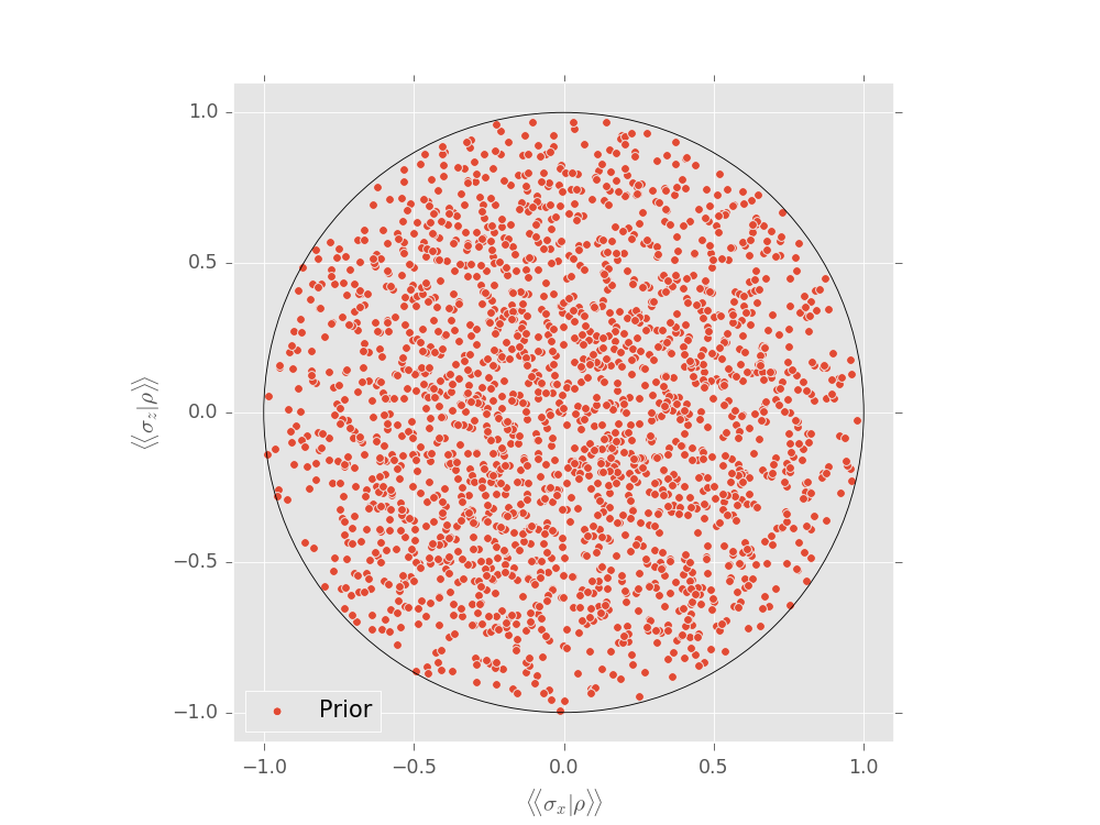
Recall this is this representation of of a qubit in the Pauli basis defined above. Quantum states are in general high dimensional objects which makes visualizing distributions of them challenging. The only 2-dimensional example is that of a rebit, which is usually defined as a qubit in the Pauli (or Bloch) representation with one of the Pauli expectations constrained to zero (usually \(\operatorname{Tr}(\rho \sigma_y)=0\)).
Here we create a distribution of rebits accord to the Ginibre ensemble and use plot_rebit_prior() to depict this distribution through (by default) 2000 random samples. While discussing models below, we will see how to depict the particles of an SMCUpdater directly.
basis = tomography.bases.pauli_basis(1)
prior = tomography.distributions.GinibreDistribution(basis)
tomography.plot_rebit_prior(prior, rebit_axes=[1, 3])
plt.show()
(Source code, svg, pdf, hires.png, png)
Using TomographyModel
The core of the tomography module is the TomographyModel. The key assumption in the current version is that of two-outcome measurements. This has the convenience of allowing experiments to be specified by a single vectorized positive operator:
>>> from qinfer.tomography import TomographyModel
>>> model = TomographyModel(basis)
>>> print(model.expparams_dtype)
[('meas', <type 'float'>, 4)]
Suppose we measure \(\sigma_z\) on a random state. The measurement effects are \(\frac12 (I\pm \sigma_z)\). Since they sum to identity, we need only specify one of them. We can use TomographyModel to calculate the Born rule probability of obtaining one of these outcomes as follows:
>>> expparams = np.zeros((1,), dtype=model.expparams_dtype)
>>> expparams['meas'][0, :] = basis.state_to_modelparams(np.sqrt(2)*(basis[0]+basis[1])/2)
>>> print(model.likelihood(0, prior.sample(), expparams))
[[[ 0.62219803]]]
Built-in Heuristics
In addition to analyzing given data sets, the tomography module is well suited for testing measurement strategies against standard heuristics. These built-in heuristics are listed at Abstract Heuristics. For qubits, the most commonly used heuristic is the random sampling of Pauli basis measurements, which is implemented by RandomPauliHeuristic.
>>> from qinfer.tomography import RandomPauliHeuristic
>>> from qinfer import SMCUpdater
>>> updater = SMCUpdater(model, 100, prior)
>>> heuristic = RandomPauliHeuristic(updater)
>>> print(model.simulate_experiment(prior.sample(), heuristic()))
0