Learning Time-Dependent Models
Time-Dependent Parameters
In addition to learning static parameters, QInfer can be used to learn the values of parameters that change stochastically as a function of time. In this case, the model parameter vector \(\vec{x}\) is interpreted as a time-dependent vector \(\vec{x}(t)\) representing the state of an underlying process. The resulting statistical problem is often referred to as state-space estimation. By using an appropriate resampling algorithm, such as the Liu-West algorithm [LW01], state-space and static parameter estimation can be combined such that a subset of the components of \(\vec{x}\) are allowed to vary with time.
QInfer represents state-space filtering by the use of
the Simulatable.update_timestep() method, which samples
how a model parameter vector is updated as a function of time.
In particular, this method is used by SMCUpdater to draw samples from the
distribution \(f\)
where \(t_{\ell}\) is the time at which the experiment \(e_{\ell}\)
is measured, and where \(t_{\ell+1}\) is the time step immediately
following \(t_{\ell}\). As this distribution is in general dependent
on the experiment being performed, update_timestep()
is vectorized in a manner similar to likelihood() (see
Designing and Using Models for details). That is,
given a tensor \(X_{i,j}\) of model parameter vectors and a vector
\(e_k\) of experiments,
update_timestep() returns a tensor \(X_{i,j,k}'\)
of sampled model parameters at the next time step.
Random Walk Models
As an example, RandomWalkModel implements update_timestep()
by taking as an input a Distribution specifying steps
\(\Delta \vec{x} = \vec{x}(t + \delta t) - \vec{x}(t)\). An
instance of RandomWalkModel decorates another model in
a similar fashion to other derived models.
For instance, the following code declares a precession model in
which the unknown frequency \(\omega\) changes by a normal
random variable with mean 0 and standard deviation 0.005 after
each measurement.
>>> from qinfer import (
...     SimplePrecessionModel, RandomWalkModel, NormalDistribution
... )
>>> model = RandomWalkModel(
...     underlying_model=SimplePrecessionModel(),
...     step_distribution=NormalDistribution(0, 0.005 ** 2)
... )
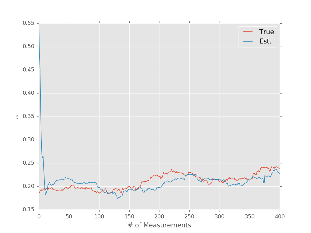
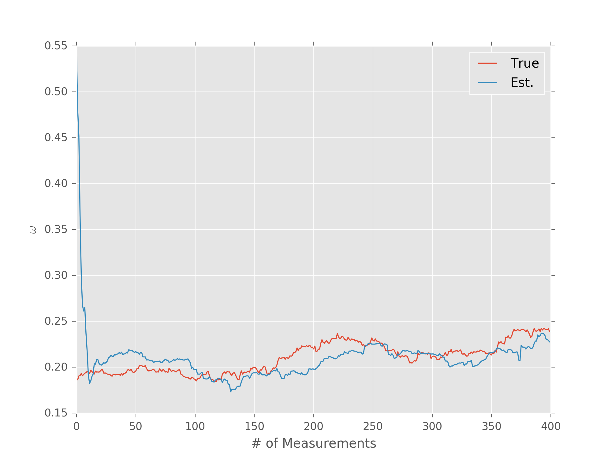
We can then draw simulated trajectories for the true and estimated value of \(\omega\) using a minor modification to the updater loop discussed in Sequential Monte Carlo.
model = RandomWalkModel(
    # Note that we set a minimum frequency of negative
    # infinity to prevent problems if the random walk
    # causes omega to cross zero.
    underlying_model=SimplePrecessionModel(min_freq=-np.inf),
    step_distribution=NormalDistribution(0, 0.005 ** 2)
)
prior = UniformDistribution([0, 1])
updater = SMCUpdater(model, 2000, prior)

expparams = np.empty((1, ), dtype=model.expparams_dtype)

true_trajectory = []
est_trajectory = []

true_params = prior.sample()

for idx_exp in range(400):
    # We don't want to grow the evolution time to be arbitrarily
    # large, so we'll instead choose a random time up to some
    # maximum.
    expparams[0] = np.random.random() * 10 * np.pi
    datum = model.simulate_experiment(true_params, expparams)
    updater.update(datum, expparams)

    # We index by [:, :, 0] to pull off the index corresponding
    # to experiment parameters.
    true_params = model.update_timestep(true_params, expparams)[:, :, 0]

    true_trajectory.append(true_params[0])
    est_trajectory.append(updater.est_mean())

plt.plot(true_trajectory, label='True')
plt.plot(est_trajectory, label='Est.')
plt.legend()
plt.xlabel('# of Measurements')
plt.ylabel(r'$\omega$')

plt.show()
(Source code, svg, pdf, hires.png, png)

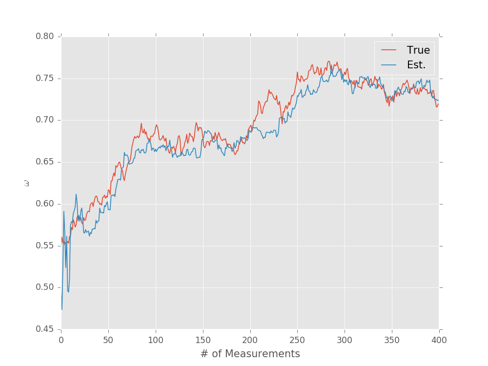
Specifying Custom Time-Step Updates
The RandomWalkModel example above is somewhat unrealistic,
however, in that the step distribution is independent of the evolution
time. For a more reasonable noise process, we would expect that
\(\mathbb{V}[\omega(t + \Delta t) - \omega(t)] \propto \Delta t\).
We can subclass SimplePrecessionModel to add this behavior
with a custom update_timestep() implementation.
class DiffusivePrecessionModel(SimplePrecessionModel):
    diffusion_rate = 0.0005 # We'll multiply this by
                             # sqrt(time) below.

    def update_timestep(self, modelparams, expparams):
        step_std_dev = self.diffusion_rate * np.sqrt(expparams)
        steps = step_std_dev * np.random.randn(
            # We want the shape of the steps in omega
            # to match the input model parameter and experiment
            # parameter shapes.
            # The axis of length 1 represents that this model
            # has only one model parameter (omega).
            modelparams.shape[0], 1, expparams.shape[0]
        )
        # Finally, we add a new axis to the input model parameters
        # to match the experiment parameters.
        return modelparams[:, :, np.newaxis] + steps

model = DiffusivePrecessionModel()
prior = UniformDistribution([0, 1])
updater = SMCUpdater(model, 2000, prior)

expparams = np.empty((1, ), dtype=model.expparams_dtype)

true_trajectory = []
est_trajectory = []

true_params = prior.sample()

for idx_exp in range(400):
    expparams[0] = np.random.random() * 10 * np.pi
    datum = model.simulate_experiment(true_params, expparams)
    updater.update(datum, expparams)

    true_params = model.update_timestep(true_params, expparams)[:, :, 0]

    true_trajectory.append(true_params[0])
    est_trajectory.append(updater.est_mean())

plt.plot(true_trajectory, label='True')
plt.plot(est_trajectory, label='Est.')
plt.legend()
plt.xlabel('# of Measurements')
plt.ylabel(r'$\omega$')

plt.show()
(Source code, svg, pdf, hires.png, png)